1
2
3
4
5
6
7
8
9
10
11
12
13
14
15
16
17
18
19
20
21
22
23
24
25
26
27
28
29
30
31
32
33
34
35
36
37
38
39
40
41
42
43
44
45
46
47
48
49
50
51
52
53
54
55
56
57
58
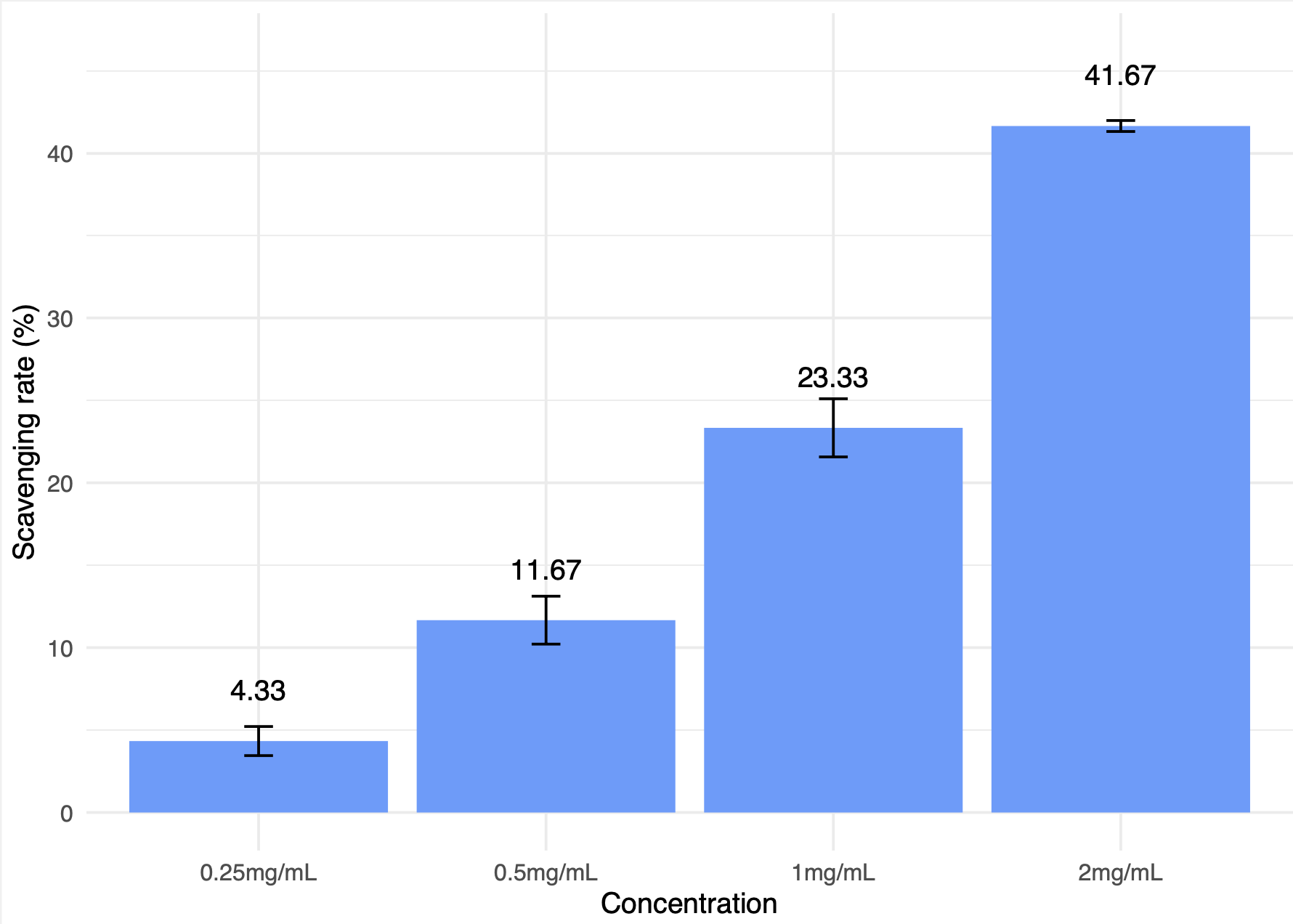
| library(ggplot2)
library(dplyr)
library(tidyr)
\# Creating the initial data frame
data <- tibble(
`0.25mg/mL` = c(6, 3, 4),
`0.5mg/mL` = c(14, 9, 12),
`1mg/mL` = c(26, 20, 24),
`2mg/mL` = c(41, 42, 42)
)
\# Calculating means and SEMs for each concentration
data_means_sems <- data %>%
summarise(across(everything(), list(mean = ~mean(.), sem = ~sd(.) / sqrt(n())))) %>%
pivot_longer(cols = everything(), names_to = "concentration_stat", values_to = "value") %>%
separate(concentration_stat, into = c("concentration", "stat"), sep = "_") %>%
pivot_wider(names_from = "stat", values_from = "value")
\# Plot with specified "skyblue" fill color and adding data labels
p <- ggplot(data_means_sems, aes(x = concentration, y = mean)) +
geom_bar(stat = "identity", position = position_dodge(), fill = "#619CFF") + # Specified fill color here
geom_errorbar(aes(ymin = mean - sem, ymax = mean + sem), width = .1) +
geom_text(aes(label = sprintf("%.2f", mean)), vjust = -2, color = "black") + # Adding mean data labels
labs(x = "Concentration", y = "Scavenging rate (%)") +
theme_minimal() +
theme(legend.position = "none")+
scale_y_continuous(limits = c(NA, max(data_means_sems$mean + data_means_sems$sem) * 1.1)) # 调整Y轴范围
print(p)
|